Initiatives – PPSM

Real-world applications of impact analysis using prediction-based propensity score matching 

Introduction

There is no shortage of interventions designed to influence our decisions and behaviors. In student nudging, we attempt to influence student behaviors associated with positive outcomes by sending automated or manual nudges at appropriate times to facilitate micro-habit formation. In student outreach through advisors or faculty, we rely on various triggers and use multiple modalities – in person, phone, email, SMS, or push notifications – to engage and motivate students in an attempt to alter future trajectories toward a more favorable direction. 

The above intervention scenario has multiple dimensions to consider. First of all, whom do you reach out to and why? When or where? Moreover, how and with what modality should institutional staff reach out to students? These questions are important given that there are so many experiment design considerations that can influence outcomes. To complicate matters even more, not all student factors that influence outcomes can be measured, i.e., confounders. Typical confounders encompass social and psychological factors, life issues, and mental/physical wellness. 

To avoid bias from confounding factors, randomized controlled trials (RCTs) have been deemed the gold standard in causal impact analysis. However, there are a few challenges with RCTs. 

The first issue is that RCTs are expensive to administer, requiring Institutional Review Board (IRB) approvals (Sabatine, 2011). They are also difficult to maintain, especially when attrition rates are high and unbalanced between pilot and control. Unless RCTs are designed in a two-arm, double-blind experiment, just the disappointment of not being selected for treatment or pilot can have unanticipated consequences in students randomly assigned to control. This disappointment is particularly acute when participants’ preference for RCT is very low and their desire to be included in the treatment arm very high (Vercellini et al., 2015; Lindstrom et al., 2010). 

The second issue is that, provided that treatment does no harm, it may be unethical to withhold treatment. While some may argue that this is a necessary sacrifice for the greater good of scientific research, there are other detractors calling for a better, more humane, and cost-effective impact measurement strategy through observational studies. 

Finally, since randomization does not perform explicit matching, RCTs are not appropriate for drill-down impact analysis for various segments of the student population, for example determining the impact differences between first-year students and continuing students. These observations led Rubin (2008) to say, “for gold standard answers, complete randomization may not be good enough, except for point estimation for very large experiments.” In student success science, prediction without action is an exercise in futility. While prediction is an important part of student success science, understanding impact elasticity – levers to pull in order to impact student success as a function of student segments and treatment strategies – is even more important. 

At Civitas Learning, we have been tackling these issues head-on and this whitepaper highlights the first part of this endeavor: matching pilot and control students in observational studies to provide intervention insights. 

Covariate matching

In quasi-experimental design (QED), baseline equivalence must be established. That is, we must find, from a control pool, students who match pilot students in some statistical sense right before pilot commencement. For student k, we make measurements as a function of time, xk(t), which can encompass cumulative GPA, prior-term GPA, credits earned ratio, high school class percentile, ACT score, Pell grant per credit, the number of credit hours attempted, etc. The covariate matching (CVM) method finds another student j, such that xj(t)≈xk(t), t = baseline. 

Since matching in a high-dimensional space becomes progressively more difficult, we use a metric called Mahalanobis distance. The Mahalanobis distance between students j and k is defined as xk-xjTR-1xk-xj, where R is the covariance matrix of a column vector x from pooled observations of x. This distance metric allows us to perform matching in a single distance metric space.  That is, for each pilot student, we compute distance metrics between the pilot student and all students in the control pool, selecting the control student with the nearest distance less than a threshold. 

Primer on propensity score matching

Propensity score matching (PSM) is a model-based approach to reducing the matching-covariate dimension by compressing high-dimensional covariates (x) into a single-dimensional metric called propensity score or p(z=1|x), where z is the treatment or program participation variable (Rosenbaum and Rubin, 1983). In essence, we use parametric (logistic regression) or nonparametric (classification and regression tree or random forest) learning algorithms to compute p(z|x), the conditional probability of a student participating in treatment, i.e., z = 1, given covariates x. PSM works by finding pilot-control pairs, where p(z|xpilot)≈p(z|xcontrol) for each pilot and matched control student. 

Rosenbaum and Rubin (1985) reviewed several multivariate matching algorithms using (1) propensity score, (2) Mahalanobis distance including propensity score, and (3) a hybrid nested method that combined propensity score and Mahalanobis distance sequentially. Their performance metric was covariate imbalance. They found that the first approach, propensity score matching, was able to reduce covariate imbalance while being the most computationally efficient. The second approach left propensity scores imbalanced between pilot and control. The third hybrid approach appeared superior to the first, albeit at the expense of computation. 

Unfortunately, none of these methods address the most important issue: what covariates to include in matching. For example, if we match on covariates that have little influence on student success outcomes, can we say that the matching was done well and that the difference in outcomes between pilot and control should be attributed to treatment? Some may argue that we should not include such knowledge in the matching process. However, if we know key success factors through historical data mining, wouldn’t it be better if matching was done on the key factors that truly influence success? 

Extending Propensity Score Matching (PSM): Prediction-Based PSM 

The prediction-based PSM (PPSM) method was developed in response to the ‘which-covariate-to-use-in-matching’ question in healthcare (Kil, Shin, and Pottschmidt, 2004). We wanted to apply salient concepts in machine learning and statistics to impact analysis, realizing that propensity score is but a prediction score of receiving treatment. In machine learning, we take pains to build robust models with high predictive accuracy and good calibration properties. Here, calibration is represented in the predictive ratio, defined as the ratio of the actual success rate to the mean predicted success rate for a group of students. Figure 1 shows the standard three plots that characterize the model performance. 

Figure 1: The three standard model performance plots – receiver operating characteristic (ROC) curves, calibration plot that shows predicted vs. actuals based on prediction-based clusters (PBC), and model bias-variance plot as a function of sample size N.. 

The central theme of PPSM is that we identify the top covariates that together maximize the predictive accuracy, and then use them in building both predictive and propensity-score models. Conceptually, matching students in propensity score using the top covariates for success ensures that pilot and control students have equal probabilities of participating in treatment. Likewise, matching students in prediction score means that pilot and control students have equal probabilities of success. Furthermore, the top covariates used in matching should exhibit good balance properties, meaning that effect size defined as covariate mean difference between pilot and control divided by pooled standard deviation should be smaller (< 0.05) after matching. The foremost reason we focus on maximizing predictive accuracy is that the higher the model accuracy, the greater the statistical power and the lower the minimum detectable effect size, as shown in Figure 2 (Kil and Shin, 2006). 

Figure 2:  This diagram illustrates the model bias-variance plot as a function of group size or N for two models with different predictive accuracies. The y-axis represents the mean and standard deviation (with an offset of 1.0) of the predictive ratio (PR) estimated from an ensemble of samples of various N’s.  As expected, the standard deviation (y-axis value – 1) decreases monotonically as a function of N, with the lower curve corresponding to the model with higher predictive accuracy measured in R-sq. The vertical black bars represent the reduction in model standard deviation attributable to improved model accuracy. 

To summarize, PPSM takes PSM one step further by adding a second dimension, px, the conditional probability of student success y given covariates x, as well as providing a mathematical rigor in selecting covariates in matching. 

Conceptually, this two-dimensional matching ensures that the matched pair of students has equal probabilities of success and intervention participation. The only difference is that one student is exposed to treatment while the other is not. Figure 3 (below) shows the two-dimensional matching process conceptually, where we match pilot and control students only if there is support in both success prediction and intervention propensity. If we cannot find support, i.e., no students with similar prediction and propensity scores, we do not match.

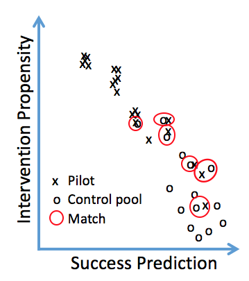
Figure 3: A conceptual picture of the two-dimensional matching in prediction and propensity scores. 

Figure 4 illustrates the methods underlying our PPSM implementation. In our case, we perform student segment-specific matching, such as new students vs. returning students, to accommodate their different digital data footprint characteristics. This data-adaptive segmentation and modeling allow us to maximize the predictive power of all available data. Covariates are then selected to maximize predictive accuracy at the point of diminishing returns, which has the added benefit of maximizing statistical power (Kil and Shin, 2006; Brookhart et al., 2006; Milliron, Malcolm, and Kil, 2014). 

First, leveraging our model-building process personalized to student segments with different data footprints, we identify top features or covariates for each student segment and each dependent variable corresponding to a student success metric. Next, we decide on a matching strategy based on how an intervention program is rolled out. If there are enough students in the same term, then we use baseline matching. If not, then we resort to mixed or pre-post matching with careful considerations given to historical student success trend stability and interference from other concurrent intervention programs. We also work with the partners on proper experiment design. 

After deciding on the matching strategy, we perform two-dimensional matching. Depending on partner request, we can also combine the two-dimensional matching with exact or Mahalanobis distance-based covariate matching. After matching, we can estimate impact numbers for the overall intervention program and for drill-down student segments and/or intervention strategies. Finally, the intervention insights are packaged and inserted into our evidence-based intervention knowledge base. 

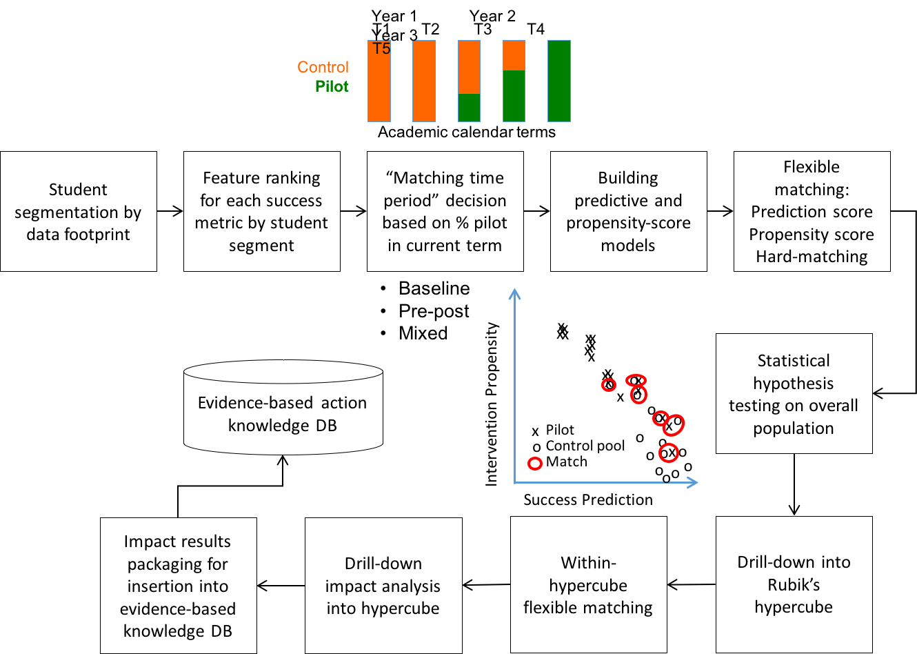
Figure 4: An illustration of Civitas Learning’s PPSM implementation. 

Finally, we need to estimate the variance of treatment effects given the model bias-variance plot in Figure 2. Since both prediction and propensity scores are estimates of student success and participation in treatment, respectively, treatment effect estimates can change based on matching algorithms, caliper widths (matching thresholds), covariates used in matching, and models used. As a result, it is always a good practice to estimate the mean and variance of treatment effects, which can be an additional consideration in making decisions based on impact analysis results. 

While there are multiple algorithms in estimating the variance of treatment effects, we use bootstrapping with no replacement for efficient computation.  (Caliendo and Kopeinig, 2008; Austin and Small, 2014).  Hill and Reiter (2006) found that confidence intervals based on the bootstrap-derived variance were more stable than other methods they investigated. Furthermore, Austin and Small (2014) found that this approach resulted in the standard error estimates very similar to the true parametric estimates of the standard error based on Monte Carlo simulations. 

Confounders and selection bias

One criticism of PSM is that it does not account for unobserved confounders, such as a student’s motivation and self-efficacy, especially in opt-in intervention programs. However, it can be argued that observed covariates may be influenced by or even accommodate these confounders. For example, one of our derived covariates, degree program alignment score, which tracks the extent to which a student follows the pathways for successful students who graduated in the same major, may encapsulate some of the student’s motivational and goal-oriented factors. Other covariates, such as grade consistency, LMS engagement, and credits earned ratio, may encompass confounders although they are not directly observable. Awan, Noureen, and Naz saw a significant relationship between achievement motivation/self-concept and academic achievement (2011). For example, when we added non-cog survey items, we found that not only did these new features not materially improve model performance but they were correlated with existing derived features.  In short, our PPSM modeling approach, leveraging derived covariates from multiple data sources, does the best possible job of dealing with selection bias and unobserved confounders. 

Attribution ambiguity with multiple, concurrent programs

A potential challenge in impact analysis is attribution ambiguity, especially when there are multiple, concurrent student success initiatives. The best approach is to decompose each student success initiative into micro pathways consisting of multiple, sequential treatments. 

Unfortunately, such passive sensing is rarely available except in limited studies, such as the Dartmouth SmartGPA project (Wang et al., 2015) and in healthcare (Phan, Kil, Piniewski, and Dou, 2016). While we intend to address such micro pathway-driven impact analysis in later papers, here we focus on program-level analysis only. This section provides a conceptual framework on how we deal with such attribution ambiguity. 

The first process is to create a temporal view of all student success initiatives as shown in Figure 5 in order to understand which programs have overlaps in time and students.

Figure 5: A time-series view of student success initiatives, where various intervention programs are overlaid over time. The y axis represents various intervention programs. 

Creating such an intervention time-series map is a prerequisite for doing impact analysis to untangle the impacts of multiple, concurrent programs. We first identify subsets of intervention programs with overlaps in time and student coverage. For each subset, we perform the following analysis outlined in Figure 6: 

1. Compute the analysis complexity score of each intervention program.
   1. Create a Venn diagram of students exposed to multiple intervention programs. 
   2. Characterize each program in terms of N, participation data availability (eligibility only or actual participation data with accurate timestamp), and time-matching mode, i.e., baseline, pre-post, or mixed. 
   3. Compute a metric for analysis complexity using heuristics. 
2. Perform marginal impact analysis for each intervention, starting from simple to complex. 
3. Ignore the interventions that do not have statistically significant impact results. 
4. For the surviving intervention programs A, B, and C, create a set of indicator variables associated with overlapping regions in Venn diagrams. 
   1. In PPSM, use these indicator variables as inputs to the matching process, i.e., covariates in prediction and propensity-score models since hard matching on the indicator variables tend to substantially reduce statistical power. 
   2. Another option is to use hierarchical linear modeling (HLM) with dosage or multiple-intervention indicator variables. 

Figure 6: Steps to minimize performance ambiguity associated with multiple, concurrent student success initiatives. 

Nevertheless, measuring intervention impact with no attribution ambiguity is very difficult and still remains a hot research topic. As a result, we have been developing exposure-to-treatment (ETT) or dynamic treatment impact analysis through dynamical PPSM (Label et al., 2014), along with key performance indicator (KPI)-engagement trigger mapping, to provide faster intervention insights with less interference from concurrent treatments. In ETT and KPI-driven impact analyses, anyone exposed to treatment (outreach event) or trigger-based nudging belongs to pilot around the treatment timestamp since most micro-interventions are assumed to have a short timespan of influence.  This framework allows us to overcome difficulties associated with measuring impact numbers in the presence of concurrent interventions. These topics will be discussed fully in subsequent white papers. 

Summary

Determining the real impact of an intervention is a difficult challenge for most institutions, particularly with RCTs often being not feasible.   With the PPSM implementation in the Civitas Student Success Platform, institutions can measure the impact of their interventions in a statistically rigorous manner that minimizes selection bias and unobserved confounding factors.  In addition, our divide-and-conquer approach combined with multi-tier dynamical impact analyses has been designed to provide more timely intervention insights with less attribution ambiguity.

References

1. M. Sabatine, “Randomized, Controlled Trials,” Circulation, Vol. 124, No. 24, Dec 2011. 
2. P. Vercellini et al., “You can’t always get what you want: from doctrine to practicality of study designs for clinical investigation in endometriosis,” BMC Women’s Health, Vol. 15, No. 19, 2015. 
3. D. Lindstrom, I. Sundberg-Petersson, J. Adami, and H. Tonnesen, “Disappointment and drop-out rate after being allocated to control group in a smoking cessation trial,” Contemporary Clinical Trials, Vol. 31, Issue 1, Jan 2010. 
4. D. Rubin, “Comment: The Design and Analysis of Gold Standard Randomized Experiments,” J. American Statistical Association, Vol. 2, No. 3, 2008. 
5. P. Rosenbaum and D. Rubin, “The central role of the propensity score in observational studies for causal effects,” Biometrika, Vol. 70, No. 1, 1983. 
6. P. Rosenbaum and D. Rubin, “Constructing a Control Group Using Multivariate Matched Sampling Methods That Incorporate the Propensity Score,” The American Statistician, Vol. 39, No. 1, 1985. 
7. D. Kil, F. Shin, and D. Pottschmidt, “Propensity Score Primer with Extensions to Propensity Score Shaping and Dynamic Impact Analysis,” Disease Management Association of America Conference, Orlando, FL, Oct 2014. 
8. M.A. Brookhart et al., “Variable Selection for Propensity Score Models,” Am. J. Epidemiology, Vol. 163, No. 12, April 2006.
9. D. Kil and F. Shin, “Utilizing Predictive Models and Integrated Data Assets to Achieve Behavioral Change and Predictable Outcomes,” 3^rd Annual Predictive Modeling Conference on Harnessing the Power of Predictive Modeling, Orlando, FL, Feb 2006.
10. M. Milliron, L. Malcolm, and D. Kil, “Insight and Action Analytics: Three Case Studies to Consider,” J. of Research and Practice in Assessment, Special Issue: Big Data and Learning Analytics, Nov 2014. 
11. M. Caliendo and S. Kopeinig, “Some Practical Guidance for the Implementation of Propensity Score Matching,” J. Economic Surveys, Vol 22. No. 1, 2008. 
12. P. Austin and D. Small, “The use of bootstrapping when using propensity-score matching without replacement: a simulation study,” Stats in Medicine, Vol. 33, 2014. 
13. R. Awan, G. Noureen, and A. Naz, “A Study of Relationships between Achievement Motivation, Self-Concept and Achievement in English and Mathematics at the Secondary Level,” International Educational Studies, Vol. 4, No. 3, Aug 2011. 
14. R. Wang, et al., “SmartGPA: How Smartphones Can Assess and Predict Student Academic Performance,” ACM Conference on Ubiquitous Computing, Osaka, Japan, Sept 2015. 
15. N. Phan. D. Kil, B. Piniewski, and D. Dou, “Next Generation Digital Therapeutics: Social and Motivational Factors for the Spread of Healthy Behavior in Social Networks,” submitted to the NEJM, Aug 2016. 
16. E. Laber, D. Lizotte, M. Quan. W. Pelham, and S. Murphy, “Dynamic treatment regimes: Technical challenges and applications,” Electronic Journal of Statistics, Vol. 8, 2014.

Was this article helpful?

0 0

How can we improve this article?

Please submit the reason for your vote so that we can improve the article.

Submit